Toolpath interpolation
![]()
Interpolation
Interpolation is a group of algorithms with the goal to compute a smooth and gradual change of a toolpath element axis. The interpolation can be applied on contour toolpaths (1-dimensional) or surface based toolpaths (2-dimensional).
There are several interpolation types available:
-
Cartesian interpolation for normal orientation
-
Cartesian interpolation for tangent orientation
-
Cartesian interpolation for offset position
-
External axis value interpolation
-
Jolt optimization (C-axis) for machines
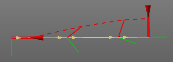
The Cartesian interpolation supports two different modes: absolute and relative interpolation. An applied interpolation can be switched between these modes which initiates an automatic recalculation of the interpolation.
For each tool path element within the interpolation interval, the proportional value for the modification (displacement or rotation) is calculated. In the absolute interpolation, the proportional value will be applied using the global coordinate system as reference.
 |  | |
| Start | Absolute interpolation |
With a relative interpolation the proportional value will be applied using the tool path element’s original local position and orientation as reference. It means that a relative interpolation does only have effect when at least one position within the interpolation range has been taught, i.e. has a modified orientation.
|  | |
| Start | Relative interpolation |
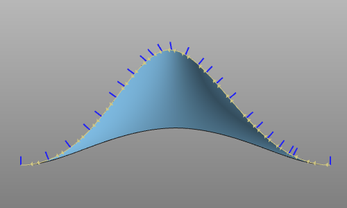
The normal interpolation method interpolates the (blue) normal directions of the toolpath positions. It will gradually rotate the normal direction from the one at the start of the interpolation range towards the direction at the end of the range so that the angle between the individual normals is minimal.
The rotation is done in the plane that is defined by the other two support axes of the toolpath element. The orthogonality of the axis system with interpolated normal direction is kept upright, and the direction of its tangent is determined to fulfill a condition of minimal deviation from the original tangent direction.
 |  | |
 |  | |
| Original toolpath | Normal interpolation |
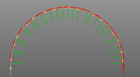
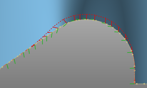
The tangent interpolation method interpolates the (red) tangent directions of the toolpath positions. It will gradually rotate the tangent direction over the normal axis from the one at the start of the interpolation range towards the direction at the end of the range so that the angle between the individual tangents is minimal.
 |  | |
| Original toolpath | Tangent interpolation |
The offset interpolation method interpolates the toolpath (offset) positions. The interpolation is calculated in the coordinate system of the base frame used for the toolpath. The deviation from an initial element position on the original toolpath is determined, and there in-between positions are calculated as their respective initial positions plus a linear combination of the support offsets. However, the combinations are chosen in such a way that the result builds a smooth curve, instead of a simple polygon.
 |  | |
| Original toolpath | Offset interpolation |
The jolt interpolation method interpolates the C-axis, sometimes also called the A-axis, rotation of the machine. It supports two modes; smooth and fix.
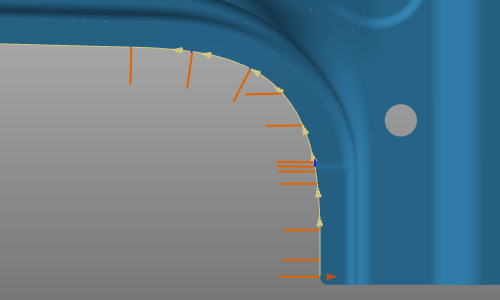
The smooth mode interpolates the axis over its interval, between the start and end position of that interval, in such a way that it changes gradually.
The fix mode sets the axis at all positions in the interval to the value of the start position.
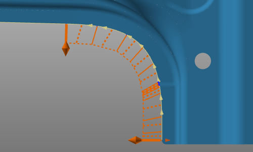 |  | |
| Smooth | Fix |
Optimization is started on a selected toolpath element. The markers of the available interpolations appear.
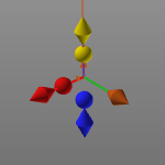
| Interpolation | Mode | Marker |
|---|---|---|
| Cartesian normal | Absolute | Blue rhombus |
| Relative | Blue sphere | |
| Cartesian tangent | Absolute | Red rhombus |
| Relative | Red sphere | |
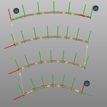
| Cartesian offset | Absolute | Yellow rhombus |
| Relative | Yellow sphere | |
| External axis value | Absolute | Brown rhombus |
| Jolt optimization | Smooth | Orange rhombus |
| Fixed | Orange sphere |
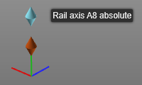
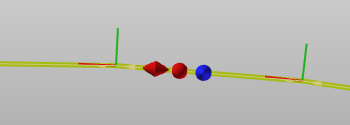
For each external axis a separate rhombus is displayed. Hovering over the rhombus indicates for which axis it applies, as shown in the example below.
After the interpolation tye has been selected, the end position is set by selecting a second toolpath element. The interpolation is calculated and the toolpath is updated.
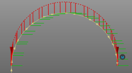
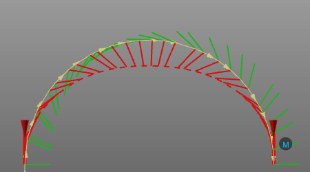
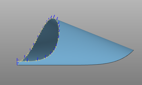
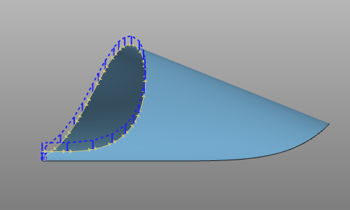
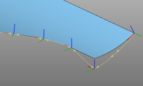
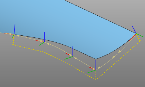
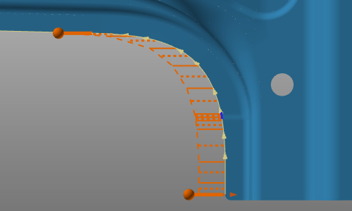
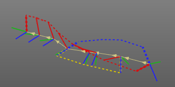
The interpolation interval is displayed as a sort of porcupine curve at the interpolated toolpath elements. The start and end position, the supports of the interpolation, are marked by a cylinder with cone end. All in the corresponding color of the interpolation type. The supports are only displayed when the interpolation is selected, i.e. active in work.
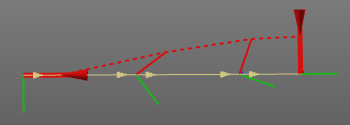
The absolute interpolation can be recognized by a dotted porcupine curve, the relative interpolation by a dashed porcupine curve.
 |  | |
| Absolute | Relative |
In between the interval, supports can be added (or deleted) to modify the interpolation. Teaching a toolpath element inside an interval will convert that element into a support of the interpolation when the taught change effects the interpolation parameter. The same applies for when a toolpath element change that effects the interpolation parameter is being removed. In that case the support is removed too. For each addition or removal of a support the interpolation is recalculated automatically.
Other modification functionality is available on the interval porcupine curve. The Pie menu can be opened here.

On manually added supports the Pie menu can be called to remove the support (not the toolpath element itself) from the interpolation.

Along a toolpath multiple interpolation intervals of different types can be created. Intervals of different interpolation types can even overlap each other.
Intervals of the same type never can overlap, only be adjacent. In that last case the interpolation remain separate; they are not merged.
Regular contour interpolation can be applied on the surface toolpath. The interval has to be defined and then the interpolation is calculated.
The surface toolpath however is built from a set of parallel tracks. The interpolation then can also be applied in a 2-dimensional approach, making use of the tracks.
Instead of a toolpath element, a track is selected to start the interpolation interval. In that case the markers appear at the track. Another track has to be selected to set the interval.
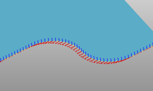
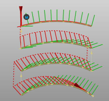
Each supporting track will be interpolated individually. Then all the tracks in between the support tracks will be interpolated proportionally using the interpolated support tracks as reference. The example below shows the effect of the 2-dimensional interpolation.
 | 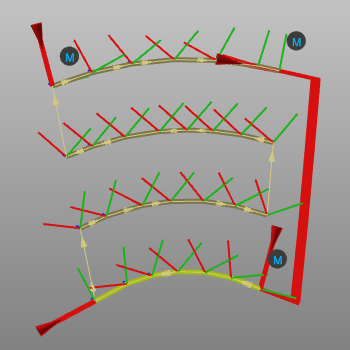 |
The interpolation interval is indicated in the color of the interpolation algorithm and covers the interval tracks.
When teaching a toolpath element on a non-support track, this track automatically becomes a support track and the interpolation is re-calculated immediately. Other modifications of the surface toolpath interpolation work the same as for contour interpolation by calling the Pie menu on the interpolation symbols.
Lead-in and lead-out are part of the track. Therefore; an interpolation over the toolpath tracks include the lead-in and -out positions.